Data Preprocessing
-
Data Gathering
Rose plots are the most popular method for plotting directional distribution data. These plots are essentially frequency histograms plotted in polar coordinates, using directional information from the total contact normal (nx, ny, nz) in the DEM simulation to illustrate particle interactions.
To facilitate connection with the CNN/CNN-GRU model, we will explore another way of presenting fabric data, namely mapping the 3D contact normal direction distribution to a 2D image. The direction value of each contact normal (nx, ny, nz) in Cartesian coordinates is converted to spherical coordinates (θ, φ). The workflow of coordinate conversion is shown in the Figure 1. The direction vector of the total contact normal can be converted using the following equation:
\(\theta = atan(\frac{\sqrt[2]{nx^2+ny^2}}{nz})\)
\(\phi = atan2(ny,nx)\)
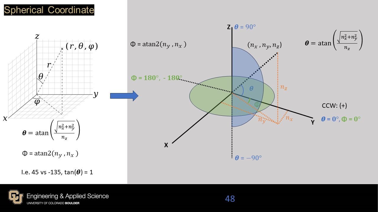
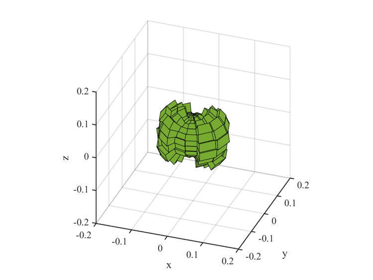
Figure 2 displays the representative rose diagram in 3D space based on cartesian coordinate.
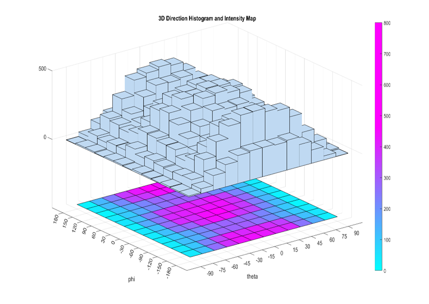
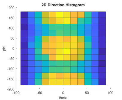
The rose diagram can be directly mapped to a frequency histogram in 3D space using converted angles (θ, ϕ) based on spherical coordinate. We can then convert these 3D histograms to 2D images by using color scale to indicate the height of each bin in the histogram. The horizontal axis represents θ within the range of [-90°, 90°], while the vertical axis corresponds to ϕ within the range of [-180°, 180°]. Figure 3 illustrates the representation of 3D directional distribution histograms and the corresponding 2D histogram images.
We can then use the top-view cross-section of 3D Histogram to construct a two-dimensional histogram of frequency to represent the direction distribution information under the contact spherical coordinate.
Open-source software YADE (Šmilauer et al, 2015) is used for all DEM simulations in this study. An assembly of 10,000 spherical particles is generated in a cubical domain using the prescribed grain size distribution (GSD). Periodic boundaries are used in the simulation to ensure that particle information is not lost due to boundary effects. Initially after generation, all particles are not in contact and are thus in a free state. Then an isotropic (or K0) consolidation procedure is performed until a target mean stress (p) value is achieved through the servo-controller set by YADE. Samples with different initial void ratios (e0) can be obtained by changing the coefficient of friction μ between particles during consolidation, and the typical μ value for quartz sand 0.5 is restored right before the shearing stage.
In this study, we prepared dense, medium, and loose samples using
\[μ_{0} = 0.0 (Dense), 0.2(Medium), 0.5(Loose)\]
The shear stage is conducted following the conventional triaxial compression condition with intermediate principal stress ratio b=0.
The magnitude of cyclic loading is determined by cyclic stress ratio , which is calculated by (deviatoric stress) and (principal stress)
\[CSR = \frac{q}{2p_{0}}\]
\[q = σ_{1}-σ_{3}\]
In this study, a CSR = 0.2 is adopted for all tests.The Cyclic Drained Triaxial Tests (Cyclic-DTX) are performed under a set of different confining pressures
\[p_{0} = 50, 100, 300, 500, 700, 1000, 1500, 2000 (kPa)\]
All tests are conducted to a maximum number of cycles (N=100). The information of stress, strain, void ratio, and fabric tensor are monitored throughout the loading program. The maximum deviatoric stress during cyclic loading is
\[q_{max}=(2p_{0})*CSR = 0.4p_{0}\]
After the cyclic loading stage, all specimens are sheared to a large value of axial strain
\[ε_{a} = 50{\\%}\]
to achieve the apparent critical state condition by monotonic loading.
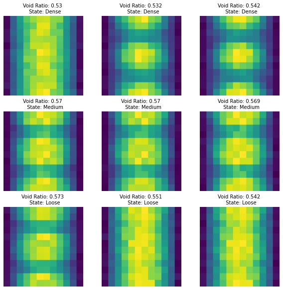
A total of 24 tests were performed and we selected void fraction information under monotonic loading, in which case the void fraction was reported as a step increase from 0% to 50% with axial strain. Therefore, we can obtain 51 two-dimensional fabric orientation distribution histogram images for each simulation, and a total of 51x24 = 1224original images are obtained through this method.
The density classification label is coded as 0, 1, and 2, and the porosity (void ratio) regression label is the real void ratio numerical data. The representative raw data is displayed in Figure 5.
| Label |
Density |
Void Ratio |
| 0 |
Dense |
Numeric(0~1) |
| 1 |
Medium |
Numeric(0~1) |
| 2 |
Loose |
Numeric(0~1) |
In order to prepare image data with a more reasonable representation, the pixel values of each input image are normalized to the range [0,1] with a scale of “(1/255.0)”. The shape of the input data is (128,128,1), which means the grayscale image is selected for prediction.
\[X_{pixel} = \frac{X_{pixel}}{255.0}\]
Clean image zipped file can be found in google drive.