Analysis
-
Models/Methods
-
CNN
A convolutional neural network (CNN) is a regularized type of feedforward neural network that learns feature engineering on its own through filter (or kernel) optimization. By using regularized weights over fewer connections, the vanishing and exploding gradients that occur during backpropagation in early neural networks can be prevented. Higher-level features are extracted from a wider context window than lower-level features.
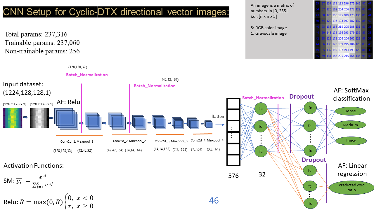
CNN models are primarily used for image processing tasks, employing a specialized technique called Convolution. Mathematically, convolution is an operation on two functions that generates a third function, illustrating how one shape is altered by the other. In the realm of deep learning, CNN models leverage this concept to process images. In this study, a deep learning model is inspired by CNN characteristics, and specifically, a two-dimensional CNN (conv2d) is utilized to discern void information in granular materials.
Typically, a CNN comprises convolutional, pooling, and fully connected layers. Any image can be characterized by its dimensions, represented as height (h) x width (w) x channels (c), with ‘channels’ denoting color information (1 for grayscale images and 3 for RGB color images). After convolution with ‘n’ kernels, the size is transformed to h x w x c x n. The kernel size aligns with the height and width of the filter, scanning the image from left to right and top to bottom with a stride ‘s’ to extract features. All values are organized in a matrix format, and matrix operations are employed to convert image features into numerical matrix information. Consequently, 2D feature maps are computed through this process. It is worth noting that during this process, the kernel may extend beyond the image boundary, and in such cases, the pixel values in that region are set to zero.
The network progresses by moving inputs forward, activating neurons positively, ultimately producing the final output. This forward movement is known as the forward pass or forward propagation. Following this, errors are computed by comparing actual data with model outputs. These errors are then propagated backward through the network, a process referred to as backpropagation. During backpropagation, to optimize the loss and achieve minimal loss, weights must be updated proportionate to their contribution to the error. This update process employs the gradient, which represents the derivative of the error with respect to the weights. A single iteration of the above process is termed an epoch. The number of epochs is determined based on the specific objectives of the work.
In general, errors can be accumulated across training examples and updated collectively at the end of a batch, a process referred to as batch learning. The batch size corresponds to the computational quantity of examples involved in each update. The extent of weight adjustment is regulated by the learning rate, often referred to as a configuration parameter or step size. The designed model are employed as outlined in Figure 1, based on the preceding information.
| Layer (type) |
Output Shape |
Param # |
Connected to |
| Input (InputLayer) |
[(None, 128, 128, 1) |
0 |
[] |
| conv2d (Conv2D) |
(None, 128, 128, 32) |
832 |
[‘Input[0][0]’] |
| batch_normalization |
(None, 128, 128, 32) |
128 |
[‘conv2d[0][0]’] |
| max_pooling2d (MaxPooling2D) |
(None, 42, 42, 32) |
0 |
[‘batch_normalization[0][0]’] |
| conv2d_1 (Conv2D) |
(None, 42, 42, 64) |
51264 |
[‘max_pooling2d[0][0]’] |
| batch_normalization_1 |
(None, 42, 42, 64) |
256 |
[‘conv2d_1[0][0]’] |
| max_pooling2d_1 (MaxPooling2D) |
(None, 14, 14, 64) |
0 |
[‘batch_normalization_1[0][0]’] |
| conv2d_2 (Conv2D) |
(None, 14, 14, 128) |
73856 |
[‘max_pooling2d_1[0][0]’] |
| max_pooling2d_2 (MaxPooling2D) |
(None, 7, 7, 128) |
0 |
[‘conv2d_2[0][0]’] |
| conv2d_3 (Conv2D) |
(None, 7, 7, 256) |
295168 |
[‘max_pooling2d_2[0][0]’] |
| max_pooling2d_3 (MaxPooling2D) |
(None, 3, 3, 256) |
0 |
[‘conv2d_3[0][0]’] |
| flatten (Flatten) |
(None, 2304) |
0 |
[‘max_pooling2d_3[0][0]’] |
| dense (Dense) |
(None, 64) |
147520 |
[‘flatten[0][0]’] |
| batch_normalization_4 |
(None, 64) |
256 |
[‘dense[0][0]’] |
| dropout (Dropout) |
(None, 64) |
0 |
[‘batch_normalization_4[0][0]’] |
| dense_1 (Dense) |
(None, 64) |
147520 |
[‘flatten[0][0]’] |
| dropout_1 (Dropout) |
(None, 64) |
0 |
[‘dropout[0][0]’] |
| dropout_2 (Dropout) |
(None, 64) |
0 |
[‘dense_1[0][0]’] |
| density (Dense) |
(None, 3) |
195 |
[‘dropout_1[0][0]’] |
| void (Dense) |
(None, 1) |
65 |
[‘dropout_2[0][0]’] |
| Total Params: 717,060 |
Trainable params: 716,740 |
Non_Trainable params: 320 |
|
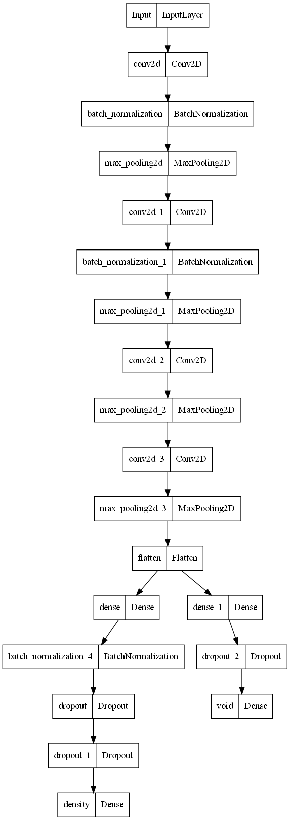
The structural details of the CNN model in TF/Keras are shown in the code section below. It is worth noting that we try to use the same model structure to implement both the classification problem and the regression problem by only changing the output layer, partial fully connected layer and dropout layer. Therefore, this CNN model does not use the traditional model.sequential() to connect the neural network structure. In a sense, the model built here is more similar to the (sequential + parallel) structure. The optimizer is Adam with a decay learning rate from 1e-4 with a decay rate of 0.9 from 10000 steps.
  ```
  inputs = Input((input_shape),name='Input')

  ## Convolutional Layers

  conv1 = Conv2D(32,kernel_size=(5,5),strides=(1,1),activation='relu',padding='same')(inputs)
  batch1 = tf.keras.layers.BatchNormalization(axis=-1,momentum=0.99,epsilon=0.009)(conv1)
  maxp1 = MaxPooling2D(pool_size=(3,3))(batch1)

  conv2 = Conv2D(64,kernel_size=(5,5),strides=(1,1),activation='relu',padding='same')(maxp1)
  batch2 = tf.keras.layers.BatchNormalization(axis=-1,momentum=0.99,epsilon=0.15)(conv2)
  maxp2 = MaxPooling2D(pool_size=(3,3))(batch2)

  conv3 = Conv2D(128,kernel_size=(3,3),strides=(1,1),activation='relu',padding='same')(maxp2)
  bacth3 = tf.keras.layers.BatchNormalization()(conv3)
  maxp3 = MaxPooling2D(pool_size=(2,2))(conv3)

  conv4 = Conv2D(256,kernel_size=(3,3),strides=(1,1),activation='relu',padding='same')(maxp3)
  batch4 = tf.keras.layers.BatchNormalization()(conv4)
  maxp4 = MaxPooling2D(pool_size=(2,2))(conv4)

  ## Flatten Layer
  flatten = Flatten()(maxp4)

  ## Fully Connected layer`

  fc1 = Dense(64,activation='relu',kernel_regularizer=tf.keras.regularizers.L2(0.09))(flatten)
  batch5 = tf.keras.layers.BatchNormalization()(fc1)
  dropout1 = Dropout(0.4)(batch5)
  fc2 = Dense(64,activation='relu')(flatten)

  dropout11 = Dropout(0.7)(dropout1)
  dropout2 = Dropout(0.05)(fc2)

  ## Regression $ Classificcation Outputs

  output1 = Dense(3,activation='softmax',name='density')(dropout11)
  output2 = Dense(1,activation='linear',name='void')(dropout2)

  model = Model(inputs = [inputs], outputs = [output1,output2])
  }
  ```
Code files can be found in github, with void ratio values (name[0]) and density labels (name[1]) written as image names.
The visualization of Model architecture is shown in Figure 2.